Slash dataset: A toy dataset that stymies most non-convolutional models.
TLDR
I’m releasing a dataset “Slash dataset” that is easy for convolutional neural nets to learn but difficult for most other models.
It will live here soph.info/data/slash_data.npz and will be licensed under a Creative Commons Attribution 4.0 International License.
Code for generating the dataset and replicating the analysis is at the bottom of this post. Cheers!
Background
The convolution is an extremely important mathematical operation. It’s frequently used in digital signal processing, including compression techniques for images and audio, and it’s the namesake and heart of “Convolutional Neural Network”.
But what actually is a convolution? There are a bunch of mesmerizing gifs like the one below, and there are some good explanations out there, but I think there’s room to improve.

I’m in the middle of a project to explain exactly what convolution does and, specifically, why it’s so useful for machine learning. As part of that effort, I’ve put together a toy dataset designed to be as simple as possible while also being difficult for all models except for convolutional ones.
Data
The dataset includes 1,000 images, each of which include a slash. It is divided into two classes according to whether the slash is downward facing (like the backslash character “”) or upward facing (like the forward slash ). Below is a random selection along with class labels.
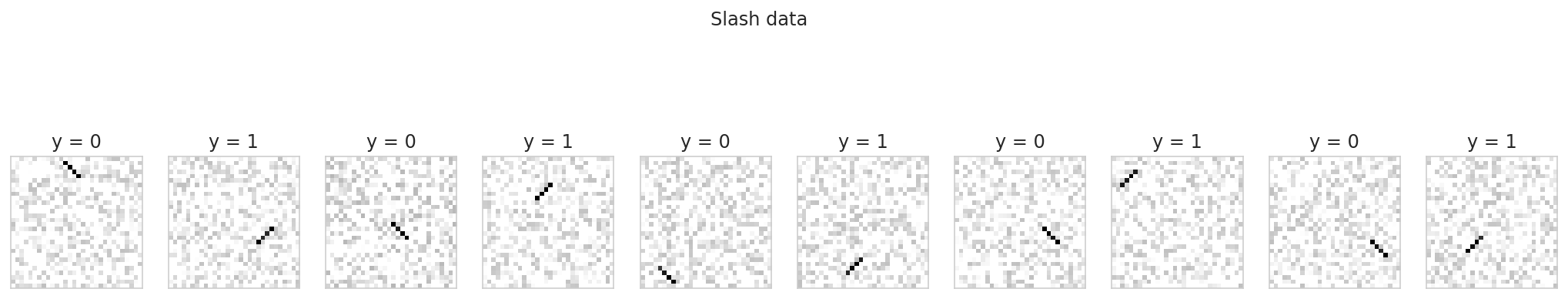
Each image is 30x30 grayscale pixels. I’ve added a little bit of noise to the images to make things interesting.
Results
| 1 | 4 | 5 | 6 | 2 | 3 | 0 | 7 | 8 | |
|---|---|---|---|---|---|---|---|---|---|
| Model | Random Forest | SVM - Linear | SVM - RBF kernel | SVM - Polynomial kernel | Logistic Regression | K Nearest Neighbors | KNN, k=1 | Vanilla CNN | Custom CNN |
| Trainable params | 9183 | 498600 | 675000 | 675000 | 901 | 675000 | 675000 | 1041 | 80 |
| Train score | 1 | 0.994667 | 0.838667 | 0.84 | 0.98 | 0.842667 | 1 | 1 | 1 |
| Test score | 0.472 | 0.5 | 0.532 | 0.532 | 0.54 | 0.604 | 0.908 | 1 | 1 |
Hopefully by now, you’re looking at this dataset and thinking “gee, that doesn’t look too difficult”. This would be a boring task for any human and it might be difficult at first to see why it is so challenging for most models.
I’m going to save a detailed explanation of exactly why that is for later. For now, I want to share my results: I tested out several off-the-shelf models as well as two convolutional models.
Of the off-the-shelf models, I didn’t waste my time tuning most of them, as I feel quite confident that even when tuned they would do poorly. (I’d love to be proved wrong on that 😉.) The one that I did tune was K-Nearest Neighbors, so you’ll see a result for one with the default parameters as well as one with the best performing parameters ($k=1$).
All of the models perform at or close enough to chance (50%) to dismiss them. KNN does pretty well when we tune it (90% test accuracy) but this performance looks less impressive when we note that KNN is memorizing the entire dataset and then comparing new examples to memorized ones. That strategy is not one that we would expect to hold up in the real world where data is much bigger than a few hundred B&W thumbnail images. Because of this, I’ve listed the trainable parameters for each model.
On the other hand, the ConvNets both get perfect scores on both train and test sets. The Vanilla CNN uses the same cookie-cutter structure that I would apply as a first attempt on just about any image data (two rounds of Convolution →Batch Normalization→Pooling). This Vanilla CNN is not tuned to the particular dataset. The Custom CNN is one I built and hand-tuned to demonstrate how ConvNets can really punch above their weight in terms of parameters. This architecture was pretty fragile (tweaking the numbers slightly is likely to break it) when testing but it’s mostly there to make a point.
Methods
All code used to generate this dataset is included below. Be on the lookout for more Convolution content shortly!